Lab 2: Data Wrangling in R
Data Wrangling
This might be the most important thing you learn about R, and about working with data. It is rare, and I daresay impossible, that the data you work on are in exactly the right form for analysis. For example, you might want to discard certain variables from the dataset to reduce clutter. Or you need to create new variables from existing ones. Or you encounter missing data. The process of gathering data in its raw form and molding it into a form that is suitable for its end use is known as data wrangling. What’s great about the tidyverse package is its suite of functions make data wrangling relatively easy, straight forward, and transparent.
In this lab, we won’t have time to go through all of the methods and functions in R that are associated with the data wrangling process. We will cover more in later labs and many methods you will have to learn on your own given the specific tasks you will need to accomplish. In the rest of this guide, we’ll go through some of the basic data wrangling techniques using the functions found in the package dplyr, which was automatically installed and loaded when you brought in the tidyverse package. These functions can be used for either tibbles or regular data frames.
Install packages
Let’s load some packages that we will need this week. We need to load
any packages we previously installed using the function
library(). Remember, install once, load every time. And if
it gives you an error for no package called..., then we
need to install those packages using install.packages(). So
when using a package, library() should always be at the top
of your R Markdown.
library(tidyverse)
library(tmap)
library(nycflights13)
Reading in data
The dataset nycflights13 was included in (Lab 1 in an R package called nycflights13. In most cases, you’ll have to read it in. Most data files you will encounter are comma-delimited (or comma-separated) files, which have .csv extensions. Comma-delimited means that columns are separated by commas. We’re going to bring in two csv files lab1dataset1.csv and lab1dataset2.csv. The first file is a county-level dataset containing median household income. The second file is also a county-level dataset containing Non-Hispanic white, Non-Hispanic black, non-Hispanic Asian, and Hispanic population counts. Both data sets come from the 2014-2018 American Community Survey (ACS). We’ll cover the Census, and how to download Census data, in another lab.
To read in a csv file, use the function read_csv(),
which is a part of the tidyverse package, and plug in
the name of the file in quotes inside the parentheses. Make sure you
include the .csv extension. The two files are up on the GitHub
for this course, so you can read them in directly from there. We’ll name
these objects ca1 and ca2.
ca1 <- read_csv("https://raw.githubusercontent.com/pjames-ucdavis/SPH215/refs/heads/main/lab1dataset1.csv")## Rows: 58 Columns: 4
## ── Column specification ────────────────────────────────────────────────────────
## Delimiter: ","
## chr (2): County, Formatted FIPS
## dbl (2): FIPS Code, Estimated median income of a household, between 2014-2018.
##
## ℹ Use `spec()` to retrieve the full column specification for this data.
## ℹ Specify the column types or set `show_col_types = FALSE` to quiet this message.ca2 <- read_csv("https://raw.githubusercontent.com/pjames-ucdavis/SPH215/refs/heads/main/lab1dataset2.csv")## Rows: 58 Columns: 12
## ── Column specification ────────────────────────────────────────────────────────
## Delimiter: ","
## chr (2): GEOID, NAME
## dbl (10): tpoprE, tpoprM, nhwhiteE, nhwhiteM, nhblkE, nhblkM, nhasnE, nhasnM...
##
## ℹ Use `spec()` to retrieve the full column specification for this data.
## ℹ Specify the column types or set `show_col_types = FALSE` to quiet this message.
You should see two tibbles ca1 and ca2 pop up in
your Environment window (top right). Every time you bring a dataset into
R for the first time, look at it to make sure you understand its
structure. You can do this a number of ways. One is to use the function
glimpse(), which gives you a succinct summary of your
data.
glimpse(ca1)## Rows: 58
## Columns: 4
## $ `FIPS Code` <dbl> 6071, 602…
## $ County <chr> "San Bern…
## $ `Formatted FIPS` <chr> "06071", …
## $ `Estimated median income of a household, between 2014-2018.` <dbl> 60164, 52…
glimpse(ca2)## Rows: 58
## Columns: 12
## $ GEOID <chr> "06033", "06047", "06043", "06049", "06013", "06027", "06099"…
## $ NAME <chr> "Lake County, California", "Merced County, California", "Mari…
## $ tpoprE <dbl> 64148, 269075, 17540, 8938, 1133247, 18085, 539301, 443738, 1…
## $ tpoprM <dbl> NA, NA, NA, NA, NA, NA, NA, NA, NA, NA, NA, NA, NA, NA, NA, N…
## $ nhwhiteE <dbl> 45623, 76008, 14125, 6962, 502951, 11389, 229796, 199356, 923…
## $ nhwhiteM <dbl> 30, 200, 31, 6, 607, 26, 445, 221, 121, 38, 980, 166, 201, 48…
## $ nhblkE <dbl> 1426, 8038, 166, 149, 93683, 160, 14338, 7881, 40, 434, 14400…
## $ nhblkM <dbl> 112, 371, 111, 97, 1433, 37, 584, 449, 47, 88, 2016, 209, 438…
## $ nhasnE <dbl> 642, 19487, 243, 130, 182135, 289, 28599, 22996, 336, 1705, 2…
## $ nhasnM <dbl> 187, 630, 95, 118, 1993, 62, 876, 507, 223, 125, 1893, 402, 6…
## $ hispE <dbl> 12830, 158494, 1909, 1292, 288101, 3927, 245973, 200060, 3866…
## $ hispM <dbl> NA, NA, NA, NA, NA, NA, NA, NA, NA, NA, NA, NA, NA, NA, NA, N…
If you like viewing your data through an Excel style worksheet, type
in View(ca1), and ca1 should pop up in the top
left window of your R Studio interface. Scroll up and down, left and
right.
We’ll learn how to summarize your data using descriptive statistics and graphs in the next lab.
By learning how to read in data the tidy way, I think you’ve earned
another badge! Woot woot! 
Renaming variables
More often than you think, you will encounter a column / variable
with a name that is not descriptive. The more descriptive the variable
names, the more efficient your analysis will be and the less likely you
are going to make a mistake. To see the names of variables in your
dataset, use the names() command.
names(ca1)## [1] "FIPS Code"
## [2] "County"
## [3] "Formatted FIPS"
## [4] "Estimated median income of a household, between 2014-2018."
The name Estimated median income of a household, between
2014-2018. is a doozy! Just a little long. Use the command
rename() to – you guessed it – rename a variable! Let’s
rename Estimated median income of a household, between
2014-2018. to medinc.
rename(ca1, medinc = "Estimated median income of a household, between 2014-2018.")## # A tibble: 58 × 4
## `FIPS Code` County `Formatted FIPS` medinc
## <dbl> <chr> <chr> <dbl>
## 1 6071 San Bernardino 06071 60164
## 2 6027 Inyo 06027 52874
## 3 6029 Kern 06029 52479
## 4 6093 Siskiyou 06093 44200
## 5 6065 Riverside 06065 63948
## 6 6019 Fresno 06019 51261
## 7 6035 Lassen 06035 56362
## 8 6049 Modoc 06049 45149
## 9 6107 Tulare 06107 47518
## 10 6023 Humboldt 06023 45528
## # ℹ 48 more rows
Note that you can rename multiple variables within the same
rename() command. For example, we can also rename
Formatted FIPS to GEOID. Make this permanent by
assigning it back to ca1 using the arrow operator
<-
ca1 <- rename(ca1,
        medinc = "Estimated median income of a household, between 2014-2018.",
        GEOID = "Formatted FIPS")
names(ca1)
## [1] "FIPS Code" "County" "GEOID" "medinc"And we can see our variable names have changed! We are doing things.
Selecting variables
In practice, most of the data files you will download will contain
variables you don’t need. It is easier to work with a smaller dataset as
it reduces clutter and clears up memory space, which is important if you
are executing complex tasks on a large number of observations. Use the
command select() to keep variables by name. Visually, we
are doing the following (taken from the RStudio cheatsheet).

Let’s take a look at the variables we have in the ca2 dataset.
names(ca2)## [1] "GEOID" "NAME" "tpoprE" "tpoprM" "nhwhiteE" "nhwhiteM"
## [7] "nhblkE" "nhblkM" "nhasnE" "nhasnM" "hispE" "hispM"We’ll go into more detail what these variables mean in another lab when we cover the U.S. Census, but we only want to keep the variables GEOID, which is the county FIPS code (a unique numeric identifier), and tpoprE, nhwhiteE, nhblkE, nhasnE, and hispE, which are the total, white, black, Asian and Hispanic population counts.
ca2 <- select(ca2, GEOID, tpoprE, nhwhiteE, nhblkE, nhasnE, hispE)
Here, we provide the data object first, followed by the variables we want to keep separated by commas.
Let’s keep County, GEOID, and medinc from
the ca1 dataset. Rather than listing all the variables we want
to keep like we did above, a shortcut way of doing this is to use the
: operator.
select(ca1, County:medinc)## # A tibble: 58 × 3
## County GEOID medinc
## <chr> <chr> <dbl>
## 1 San Bernardino 06071 60164
## 2 Inyo 06027 52874
## 3 Kern 06029 52479
## 4 Siskiyou 06093 44200
## 5 Riverside 06065 63948
## 6 Fresno 06019 51261
## 7 Lassen 06035 56362
## 8 Modoc 06049 45149
## 9 Tulare 06107 47518
## 10 Humboldt 06023 45528
## # ℹ 48 more rows
The : operator tells R to select all the variables from
County to medinc. This operator is useful when you’ve
got a lot of variables to keep and they all happen to be ordered
sequentially.
You can use also use select() command to keep variables
except for the ones you designate. For example, to keep all variables in
ca1 except FIPS Code and save this back into
ca1, type in:
ca1 <- select(ca1, -"FIPS Code")
The negative sign tells R to exclude the variable. Notice we need to
use quotes around FIPS Code because it contains a space. You
can delete multiple variables. For example, if you wanted to keep all
variables except FIPS Code and County, you would type
in select(ca1, -"FIPS Code", -County).
Take a glimpse and see if it looks how we think it should.
glimpse(ca1)## Rows: 58
## Columns: 3
## $ County <chr> "San Bernardino", "Inyo", "Kern", "Siskiyou", "Riverside", "Fre…
## $ GEOID <chr> "06071", "06027", "06029", "06093", "06065", "06019", "06035", …
## $ medinc <dbl> 60164, 52874, 52479, 44200, 63948, 51261, 56362, 45149, 47518, …Try ca2 and let us know how it looks.
Creating new variables
The mutate() function (strange name, huh?) allows you to
create new variables within your dataset. This is important when you
need to transform variables in some way - for example, calculating a
ratio or adding two variables together. Visually, you are doing this:
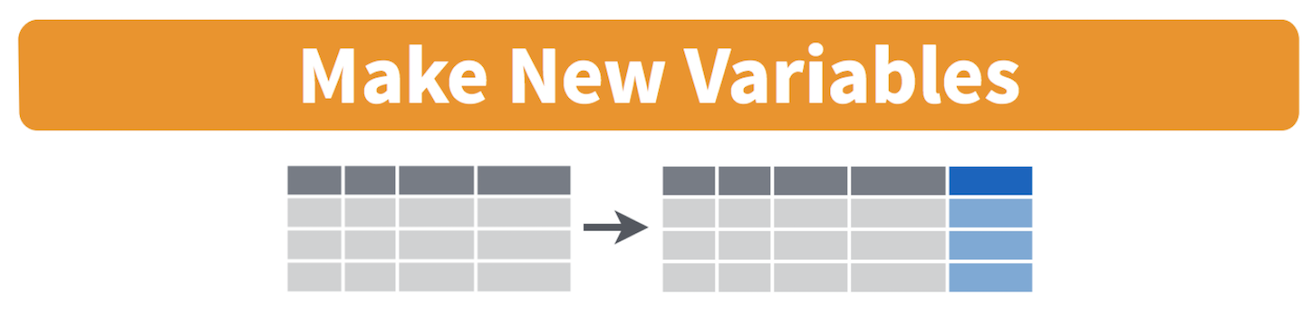
You can use the mutate() command to generate as many new
variables as you would like. For example, let’s construct four new
variables in ca2 - the percent of residents who are
non-Hispanic white, non-Hispanic Asian, non-Hispanic black, and
Hispanic. Name these variables pwhite, pasian,
pblack, and phisp, respectively.
mutate(ca2, pwhite = nhwhiteE/tpoprE, pasian = nhasnE/tpoprE,
              pblack = nhblkE/tpoprE, phisp = hispE/tpoprE)
## # A tibble: 58 × 10
## GEOID tpoprE nhwhiteE nhblkE nhasnE hispE pwhite pasian pblack phisp
## <chr> <dbl> <dbl> <dbl> <dbl> <dbl> <dbl> <dbl> <dbl> <dbl>
## 1 06033 64148 45623 1426 642 12830 0.711 0.0100 0.0222 0.200
## 2 06047 269075 76008 8038 19487 158494 0.282 0.0724 0.0299 0.589
## 3 06043 17540 14125 166 243 1909 0.805 0.0139 0.00946 0.109
## 4 06049 8938 6962 149 130 1292 0.779 0.0145 0.0167 0.145
## 5 06013 1133247 502951 93683 182135 288101 0.444 0.161 0.0827 0.254
## 6 06027 18085 11389 160 289 3927 0.630 0.0160 0.00885 0.217
## 7 06099 539301 229796 14338 28599 245973 0.426 0.0530 0.0266 0.456
## 8 06083 443738 199356 7881 22996 200060 0.449 0.0518 0.0178 0.451
## 9 06051 14174 9234 40 336 3866 0.651 0.0237 0.00282 0.273
## 10 06069 59416 20780 434 1705 35248 0.350 0.0287 0.00730 0.593
## # ℹ 48 more rows
Note that you can create new variables based on the variables you
just created in the same line of code. For example, you can create a
categorical variable called mhisp yielding “Majority” if the
tract is majority Hispanic and “Not Majority” otherwise after creating
the percent Hispanic variable phisp within the same
mutate() command. Let’s save these changes back into
ca2.
ca2 <- mutate(ca2, pwhite = nhwhiteE/tpoprE, pasian = nhasnE/tpoprE,
              pblack = nhblkE/tpoprE, phisp = hispE/tpoprE,
              mhisp = case_when(phisp > 0.5 ~ "Majority",
                                .default = "Not Majority"))
We used the function case_when() to create
mhisp - the function tells R that if the condition
phisp > 0.5 is met, the tract’s value for the variable
mhisp will be “Majority”, otherwise (designated by
.default=) it will be “Not Majority”.
Take a look at our data. Pay attention to phisp and mhisp. Did our calculation work?
glimpse(ca2)## Rows: 58
## Columns: 11
## $ GEOID <chr> "06033", "06047", "06043", "06049", "06013", "06027", "06099"…
## $ tpoprE <dbl> 64148, 269075, 17540, 8938, 1133247, 18085, 539301, 443738, 1…
## $ nhwhiteE <dbl> 45623, 76008, 14125, 6962, 502951, 11389, 229796, 199356, 923…
## $ nhblkE <dbl> 1426, 8038, 166, 149, 93683, 160, 14338, 7881, 40, 434, 14400…
## $ nhasnE <dbl> 642, 19487, 243, 130, 182135, 289, 28599, 22996, 336, 1705, 2…
## $ hispE <dbl> 12830, 158494, 1909, 1292, 288101, 3927, 245973, 200060, 3866…
## $ pwhite <dbl> 0.7112147, 0.2824789, 0.8053022, 0.7789215, 0.4438141, 0.6297…
## $ pasian <dbl> 0.010008106, 0.072422187, 0.013854048, 0.014544641, 0.1607195…
## $ pblack <dbl> 0.022229843, 0.029872712, 0.009464082, 0.016670396, 0.0826677…
## $ phisp <dbl> 0.20000624, 0.58903280, 0.10883694, 0.14455135, 0.25422613, 0…
## $ mhisp <chr> "Not Majority", "Majority", "Not Majority", "Not Majority", "…
Joining Tables
Rather than working on two separate datasets, we should join the two datasets ca1 and ca2, because we may want to examine the relationship between median household income, which is in ca1, and racial/ethnic composition, which is in ca2. To do this, we need a unique ID that connects the tracts across the two files. The unique Census ID for a county combines the county and state IDs. The Census ID is named GEOID in both files. The IDs should be the same data class. Let’s check if they are!
class(ca1$GEOID)## [1] "character"class(ca2$GEOID)## [1] "character"
Lookin good! Note: If they are not the same class, we can coerce them
using the as.numeric() or as.character()
function described earlier.
To merge the datasets together, use the function
left_join(), which matches pairs of observations whenever
their keys or IDs are equal. We match on the variable GEOID and save the
merged data set into a new object called cacounty.
cacounty <- left_join(ca1, ca2, by = "GEOID")
We want to merge ca2 into ca1, so that’s why the
sequence is ca1, ca2. The argument by tells R
which variable(s) to match rows on, in this case GEOID. You can
match on multiple variables and you can also match on a single variable
with different variable names (see the left_join() help
documentation for how to do this). The number of columns in
cacounty equals the number of columns in ca1 plus the
number of columns in ca2 minus the ID variable you merged
on.
Note that if you have two variables with the same name in both files, R will attach a .x to the variable name in ca1 and a .y to the variable name in ca1. For example, if you have a variable named Robert in both files, cacounty will contain both variables and name it Robert.x (the variable in ca1) and Robert.y (the variable in ca1). Try to avoid having variables with the same names in the two files you want to merge.
Let’s use select() to keep the necessary variables.
cacounty <- select(cacounty, GEOID, County, pwhite, pasian, pblack, phisp, mhisp, medinc)
Filtering
Filtering means selecting rows/observations based on their values. To
filter in R, use the command filter(). Visually, filtering
rows looks like.
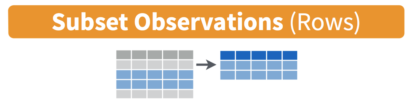 The first argument in
the parentheses of this command is the name of the data frame. The
second and any subsequent arguments (separated by commas) are the
expressions that filter the data frame. For example, we can select
Sacramento county using its FIPS
code. A FIPS code is a unique ID for every geographic unit in the
US. This will come up often!
The first argument in
the parentheses of this command is the name of the data frame. The
second and any subsequent arguments (separated by commas) are the
expressions that filter the data frame. For example, we can select
Sacramento county using its FIPS
code. A FIPS code is a unique ID for every geographic unit in the
US. This will come up often!
filter(cacounty, GEOID == "06067")## # A tibble: 1 × 8
## GEOID County pwhite pasian pblack phisp mhisp medinc
## <chr> <chr> <dbl> <dbl> <dbl> <dbl> <chr> <dbl>
## 1 06067 Sacramento 0.452 0.153 0.0954 0.230 Not Majority 63902
The double equal operator == means equal to. We can also
explicitly exclude cases and keep everything else by using the not equal
operator !=. Conversely, the following code
excludes Sacramento county.
filter(cacounty, GEOID != "06067")## # A tibble: 57 × 8
## GEOID County pwhite pasian pblack phisp mhisp medinc
## <chr> <chr> <dbl> <dbl> <dbl> <dbl> <chr> <dbl>
## 1 06071 San Bernardino 0.292 0.0682 0.0791 0.528 Majority 60164
## 2 06027 Inyo 0.630 0.0160 0.00885 0.217 Not Majority 52874
## 3 06029 Kern 0.348 0.0456 0.0510 0.528 Majority 52479
## 4 06093 Siskiyou 0.767 0.0154 0.0142 0.123 Not Majority 44200
## 5 06065 Riverside 0.359 0.0620 0.0606 0.484 Not Majority 63948
## 6 06019 Fresno 0.298 0.100 0.0455 0.527 Majority 51261
## 7 06035 Lassen 0.658 0.0140 0.0864 0.187 Not Majority 56362
## 8 06049 Modoc 0.779 0.0145 0.0167 0.145 Not Majority 45149
## 9 06107 Tulare 0.290 0.0321 0.0127 0.641 Majority 47518
## 10 06023 Humboldt 0.746 0.0298 0.00988 0.113 Not Majority 45528
## # ℹ 47 more rows
What about filtering if a county has a value greater than a specified value? For example, counties with a percent white greater than 0.5 (50%).
filter(cacounty, pwhite > 0.5)## # A tibble: 30 × 8
## GEOID County pwhite pasian pblack phisp mhisp medinc
## <chr> <chr> <dbl> <dbl> <dbl> <dbl> <chr> <dbl>
## 1 06027 Inyo 0.630 0.0160 0.00885 0.217 Not Majority 52874
## 2 06093 Siskiyou 0.767 0.0154 0.0142 0.123 Not Majority 44200
## 3 06035 Lassen 0.658 0.0140 0.0864 0.187 Not Majority 56362
## 4 06049 Modoc 0.779 0.0145 0.0167 0.145 Not Majority 45149
## 5 06023 Humboldt 0.746 0.0298 0.00988 0.113 Not Majority 45528
## 6 06089 Shasta 0.802 0.0297 0.0119 0.0983 Not Majority 50905
## 7 06045 Mendocino 0.656 0.0191 0.00585 0.248 Not Majority 49233
## 8 06105 Trinity 0.825 0.0139 0.00676 0.0723 Not Majority 38497
## 9 06079 San Luis Obispo 0.691 0.0353 0.0175 0.224 Not Majority 70699
## 10 06103 Tehama 0.687 0.0152 0.00663 0.247 Not Majority 42899
## # ℹ 20 more rows
What about less than 0.5 (50%)?
filter(cacounty, pwhite < 0.5)## # A tibble: 28 × 8
## GEOID County pwhite pasian pblack phisp mhisp medinc
## <chr> <chr> <dbl> <dbl> <dbl> <dbl> <chr> <dbl>
## 1 06071 San Bernardino 0.292 0.0682 0.0791 0.528 Majority 60164
## 2 06029 Kern 0.348 0.0456 0.0510 0.528 Majority 52479
## 3 06065 Riverside 0.359 0.0620 0.0606 0.484 Not Majority 63948
## 4 06019 Fresno 0.298 0.100 0.0455 0.527 Majority 51261
## 5 06107 Tulare 0.290 0.0321 0.0127 0.641 Majority 47518
## 6 06037 Los Angeles 0.263 0.144 0.0788 0.485 Not Majority 64251
## 7 06073 San Diego 0.459 0.116 0.0471 0.335 Not Majority 74855
## 8 06025 Imperial 0.110 0.0132 0.0217 0.838 Majority 45834
## 9 06053 Monterey 0.303 0.0546 0.0245 0.583 Majority 66676
## 10 06083 Santa Barbara 0.449 0.0518 0.0178 0.451 Not Majority 71657
## # ℹ 18 more rows
Both lines of code do not include counties that have a percent white
equal to 0.5. We include it by using the less than or equal operator
<= or greater than or equal operator
>=.
filter(cacounty, pwhite <= 0.5)## # A tibble: 28 × 8
## GEOID County pwhite pasian pblack phisp mhisp medinc
## <chr> <chr> <dbl> <dbl> <dbl> <dbl> <chr> <dbl>
## 1 06071 San Bernardino 0.292 0.0682 0.0791 0.528 Majority 60164
## 2 06029 Kern 0.348 0.0456 0.0510 0.528 Majority 52479
## 3 06065 Riverside 0.359 0.0620 0.0606 0.484 Not Majority 63948
## 4 06019 Fresno 0.298 0.100 0.0455 0.527 Majority 51261
## 5 06107 Tulare 0.290 0.0321 0.0127 0.641 Majority 47518
## 6 06037 Los Angeles 0.263 0.144 0.0788 0.485 Not Majority 64251
## 7 06073 San Diego 0.459 0.116 0.0471 0.335 Not Majority 74855
## 8 06025 Imperial 0.110 0.0132 0.0217 0.838 Majority 45834
## 9 06053 Monterey 0.303 0.0546 0.0245 0.583 Majority 66676
## 10 06083 Santa Barbara 0.449 0.0518 0.0178 0.451 Not Majority 71657
## # ℹ 18 more rows
In addition to comparison operators, filtering may also utilize
logical operators that make multiple selections. There are three basic
logical operators: & (and), | is (or), and
! is (not). We can keep counties with phisp
greater than 0.5 and medinc greater than 50000
percent using &.
filter(cacounty, phisp > 0.5 & medinc > 50000)## # A tibble: 9 × 8
## GEOID County pwhite pasian pblack phisp mhisp medinc
## <chr> <chr> <dbl> <dbl> <dbl> <dbl> <chr> <dbl>
## 1 06071 San Bernardino 0.292 0.0682 0.0791 0.528 Majority 60164
## 2 06029 Kern 0.348 0.0456 0.0510 0.528 Majority 52479
## 3 06019 Fresno 0.298 0.100 0.0455 0.527 Majority 51261
## 4 06053 Monterey 0.303 0.0546 0.0245 0.583 Majority 66676
## 5 06039 Madera 0.345 0.0197 0.0312 0.573 Majority 52884
## 6 06047 Merced 0.282 0.0724 0.0299 0.589 Majority 50129
## 7 06069 San Benito 0.350 0.0287 0.00730 0.593 Majority 81977
## 8 06031 Kings 0.327 0.0382 0.0585 0.541 Majority 53865
## 9 06011 Colusa 0.357 0.0151 0.0129 0.590 Majority 56704
Use | to keep counties with a GEOID of 06067
(Sacramento) or 06113 (Yolo) or 06075
(San Francisco).
filter(cacounty, GEOID == "06067" | GEOID == "06113" | GEOID == "06075")## # A tibble: 3 × 8
## GEOID County pwhite pasian pblack phisp mhisp medinc
## <chr> <chr> <dbl> <dbl> <dbl> <dbl> <chr> <dbl>
## 1 06113 Yolo 0.471 0.137 0.0243 0.315 Not Majority 65923
## 2 06067 Sacramento 0.452 0.153 0.0954 0.230 Not Majority 63902
## 3 06075 San Francisco 0.406 0.339 0.0501 0.152 Not Majority 104552
Phew. That’s a lot! You’ve gone through some of the basic data
wrangling functions offered by tidyverse. Can we get another Tidy badge?
Oh yeah. Congratulations! 
R Markdown
In running the lines of code above, we’ve asked you to work directly
in the R Console and issue commands in an interactive way. That is, you
type a command after >, you hit enter/return, R
responds, you type the next command, hit enter/return, R responds, and
so on. Instead of writing the command directly into the console, you
should write it in a script. The process is now: Type your command in
the script. Run the code from the script. R responds. You get results.
You can write two commands in a script. Run both simultaneously. R
responds. You get results. This is the basic flow.
One way to do this is to use the default R Script, which is covered in the assignment guidelines. In your homework assignments, we will be asking you to submit code in another type of script: the R Markdown file. R Markdown allows you to create documents that serve as a neat record of your analysis. Think of it as a word document file, but instead of sentences in an essay, you are writing code for a data analysis.
When going through lab guides, I would recommend not copying and pasting code directly into the R Console, but saving and running it in an R Markdown file. This will give you good practice in the R Markdown environment. Now is a good time to read through the class assignment guidelines as they go through the basics of R Markdown files.
To open an R Markdown file, click on File at the top menu in RStudio, select New File, and then R Markdown…. A window should pop up. In that window, for title, put in “Lab 2”. For author, put your name. Leave the HTML radio button clicked, and select OK. A new R Markdown file should pop up in the top left window.
Don’t change anything inside the YAML (the stuff at the top in
between the ---). Also keep the grey chunk after the
YAML.
Delete everything else. Save this file (File -> Save) in an appropriate folder. It’s best to set up a clean and efficient file management structure (e.g., SPH215>Labs>Lab1) but you do what works for you.
Follow the directions in the assignment guidelines to add this lab’s code in your Lab 2 R Markdown file. Then knit it as an html, word or pdf file. You don’t have to turn in the Rmd and its knitted file, but it’s good practice to create an Rmd file for each lab (and you will see that the lab assignments are eerily similar to what we do in the lab, so you will save yourself time).
Although the lab guides and course textbooks should get you through a lot of the functions that are needed to successfully accomplish tasks for this class, there are a number of useful online resources on R and RStudio that you can look into if you get stuck or want to learn more. We outline these resources in the R Help section of the website. If you ever get stuck, check this resource out first to troubleshoot before immediately asking a friend or the instructor.
Practice makes perfect
Here are a few practice questions. You don’t need to submit these, but it’s good practice to answer these questions in R Markdown, producing a knitted file (html, pdf or docx).
- Look up the help documentation for the function
rep(). Use this function to create the following 3 vectors.
- [1] 0 0 0 0 0
- [1] 1 2 3 1 2 3 1 2 3 1 2 3
- [1] 4 5 5 6 6 6
- Explain what is the problem in each line of code below. Fix the code so it will run properly.
- my variable <- 3
- seq(1, 10 by = 2)
- Library(cars)
- Look up the help documentation for the function
cut().
- Describe the purpose of this function. What kind of data type(s) does this function accept? Which arguments/options are required? Which arguments are not required and what are their default value(s)?
- Create an example vector and use the
cut()function on it. Explain your results.
Load the mtcars dataset by using the code
data(mtcars). Find the minimum, mean, median and maximum of the variable mpg in the mtcars dataset using just one line of code. We have not covered a function that does this yet, so the main point 1. of this question is to get you used to using the resources you have available to find an answer. Describe the process you used (searched online? used the class textbook?) to find the answer.Look up the functions
arrange()andrelocate(). Input the variable phisp from cacounty in each function. What are the functions doing?Use the function
bind_rows()to create a new dataset called cacounty_brows that combines ca1 and ca2. Describe the structure of this new dataset. Do the same for the functionbind_cols()(name the new dataset cacounty_bcols). How isbind_cols()different fromleft_join()?
But wait, we didn’t make a map!
This lab is a foundation for all of the work we will do moving forward in R. But what kind of GIS course would this be if we didn’t make a map? Remember that dataset we brought in earlier on cancer cases across CA called ca_cancer? Let’s plot that real quick. We will talk more about it next week (or later today if we have time)!
# Download Cancer Dataset
download.file("https://raw.githubusercontent.com/pjames-ucdavis/SPH215/refs/heads/main/CA_Cancer_Data.rds", "ca_cancer.rds", mode = "wb")

# Read in Cancer Dataset
cancer <- readRDS("ca_cancer.rds")

## Let's view the data
head(cancer)
## time event AGE INS geometry
## 1 1.275976 1 67 Mcr POINT (-122.3492 38.3025)
## 14 3.509907 1 69 Mcr POINT (-121.9832 37.82052)
## 17 10.297702 0 75 Mng POINT (-122.3092 38.3314)
## 36 7.012532 0 46 Mcr POINT (-122.2031 38.09592)
## 55 3.389200 0 70 Mcr POINT (-122.6356 38.26257)
## 92 6.110251 1 59 Unk POINT (-122.0198 37.35523)table(cancer$event)##
## 0 1
## 424 550## Load these packages--let's not worry too much about what they do!
library(sf)## Linking to GEOS 3.13.0, GDAL 3.8.5, PROJ 9.5.1; sf_use_s2() is TRUElibrary(tmap)
## Setting coordinate reference system (CRS) to North American Datum 1983 (NAD83)--we will discuss more next week!
cancer_projected = st_as_sf(cancer, crs=4269)
## Plot the data--will also discuss more in a few weeks!
tmap_mode("view")## ℹ tmap modes "plot" - "view"## ℹ toggle with `tmap::ttm()`
## This message is displayed once per session.cancer_map = tm_shape(cancer_projected) +
tm_dots(size=0.5,fill_alpha=0.8, fill="event",fill.scale = tm_scale_categorical())
cancer_mapOK we made a pretty map! Blue dots mean they didn’t have the “event” and green means they did. We are going to dive much deeper on this next week. I think this is enough for today! Get outside and enjoy the rest of your day!