Lab 9: Future Directions in GIS and Public Health

“Remember: every GPS point is a step toward understanding the world a little better.”

In this final lab, we bring together everything we’ve learned this quarter:
vector data, raster data, coordinate systems, interactive maps, and exposure science. In this lab, we’re diving into the wonderful world of GPS data, our old friend NDVI rasters, and some fun interactive mapping – with a light touch and an emphasis on public health applications. This will be our last interactive session, so we will lean on old tools we’ve been using, and we will also apply some new packages for the first time!

The objectives of this guide are to teach you to:

1. Understand how to load and preprocess GPS tracking data in R
2. Calculate movement metrics (distance + speed)
   
3. Create interactive mobility maps with leaflet
   
4. Compare spatial patterns across time of day using tmap
   
5. Integrate NDVI rasters as environmental exposure
   
6. Extract momentary exposure values
   
7. Visualize exposure over time

Let’s do this, one last time!

---

Load our packages

library(dplyr)        # data wrangling, piping, and general awesomeness
library(readr)        # reading in data like a pro
library(terra)        # handling raster data
library(sf)           # spatial vector data with all the bells and whistles
library(tmap)         # beautiful thematic maps, both static and interactive

#New Packages this week!
library(lubridate)    # working with dates and times like it's no big deal
library(leaflet)      # making interactive maps that aim to impress
library(geosphere)    # helps us to colculate the great-circle distance between two points

Import and Prepare Our GPS Data

Here we read in our GPS dataset, parse the timestamp, and create friendly time labels. This is where readr, dplyr, and lubridate come together to easily tackle this task.

download.file(
  "https://raw.githubusercontent.com/pjames-ucdavis/SPH215/refs/heads/main/gps_apr25_30.csv",
  destfile = "gps_apr25_30.csv",
  mode = "wb"
)

gps_data_raw <- read_csv("gps_apr25_30.csv")

gps_data <- gps_data_raw %>%
  mutate(
    time = ymd_hms(`UTC time`),
    time_label = format(time, "%Y-%m-%d %H:%M:%S")
  ) %>%
  arrange(time)

glimpse(gps_data)

## Rows: 21,886
## Columns: 8
## $ timestamp  <dbl> 1.61931e+12, 1.61931e+12, 1.61931e+12, 1.61931e+12, 1.61931…
## $ `UTC time` <dttm> 2021-04-25 00:15:10, 2021-04-25 00:15:10, 2021-04-25 00:16…
## $ latitude   <dbl> 42.37178, 42.37177, 42.37180, 42.37183, 42.37186, 42.37183,…
## $ longitude  <dbl> -71.08780, -71.08793, -71.08796, -71.08791, -71.08791, -71.…
## $ altitude   <dbl> 16.142262, 3.940258, 3.940258, 3.940258, 3.940258, 3.940258…
## $ accuracy   <dbl> 25.62929, 65.00000, 1030.74153, 65.00000, 65.00000, 65.0000…
## $ time       <dttm> 2021-04-25 00:15:10, 2021-04-25 00:15:10, 2021-04-25 00:16…
## $ time_label <chr> "2021-04-25 00:15:10", "2021-04-25 00:15:10", "2021-04-25 0…

We now have minute-level GPS points over multiple days.

Movement Analytics

Now we will calculate:

• Distance between consecutive points
  
• Time difference
  
• Speed

This helps us to have an idea of how fast we are moving at any point!

gps_data <- gps_data %>%
  mutate(
    lon2 = lead(longitude),
    lat2 = lead(latitude),
    t2   = lead(time),
    dt_s = as.numeric(difftime(t2, time, units = "secs")),
    step_m = distHaversine(
      cbind(longitude, latitude),
      cbind(lon2, lat2)
    ),
    speed_mps = step_m / dt_s
  ) %>%
  filter(dt_s > 0) %>%                       # remove zero/negative time gaps
  mutate(speed_mps = ifelse(is.infinite(speed_mps), NA, speed_mps))

summary(gps_data$speed_mps)

##     Min.  1st Qu.   Median     Mean  3rd Qu.     Max. 
##   0.0000   0.0000   0.0000   1.2290   0.8059 884.9334

That is a dynamic view of human mobility in meters per second. Some of those numbers are a little high though!

Mapping with Leaflet: Interactive Map Colored by Speed (mph)

Now let’s use the leaflet package to make an interactive map of our GPS data. This lets us explore movement patterns dynamically, and it’s a great way to get familiar with spatial data in a hands-on way. Let’s start off by converting speed to miles per hour and removing unrealistic values (>90 mph).

gps_speed_clean <- gps_data %>%
  mutate(speed_mph = speed_mps * 2.23694) %>%
  filter(
    !is.na(speed_mph),
    speed_mph > 0,
    speed_mph < 90
  )

Now let’s map points by speed!

pal_speed <- colorNumeric(
  palette = "viridis",
  domain = range(gps_speed_clean$speed_mph, na.rm = TRUE)
)

leaflet(gps_speed_clean) %>%
  addProviderTiles("CartoDB.Positron") %>%
  addCircleMarkers(
    lng = ~longitude,
    lat = ~latitude,
    radius = 3,
    color = ~pal_speed(speed_mph),
    stroke = FALSE,
    fillOpacity = 0.85,
    popup = ~paste(
      "Time:", time_label,
      "<br>Speed (mph):", round(speed_mph, 1)
    )
  ) %>%
  addLegend(
    "bottomright",
    pal = pal_speed,
    values = ~speed_mph,
    title = "Speed (mph)"
  )

This map shows where movement is slow (likely stationary or walking) versus fast (driving). What do we see?

---

Time-of-Day Maps

Let’s compare spatial behavior across time of day. Where did I spend time during the morning? What about afternoon and evening? What about night?

gps_data <- gps_data %>%
  mutate(
    hour = hour(time),
    tod = cut(
      hour,
      breaks = c(-1, 5, 11, 17, 23),
      labels = c("Night", "Morning", "Afternoon", "Evening")
    )
  )

gps_sf <- st_as_sf(gps_data, coords = c("longitude", "latitude"), crs = 4326)

tmap_mode("plot")

## ℹ tmap modes "plot" - "view"
## ℹ toggle with `tmap::ttm()`

tm_shape(gps_sf) +
  tm_symbols(
    fill = "steelblue",
    col = NA,
    size = 0.2,
    fill_alpha = 0.6
  ) +
  tm_facets(by = "tod", ncol = 2, free.coords = FALSE) +
  tm_title(  
    text = "Activity Space by Time of Day",
    size = 1.2,
    ) +
  tm_basemap()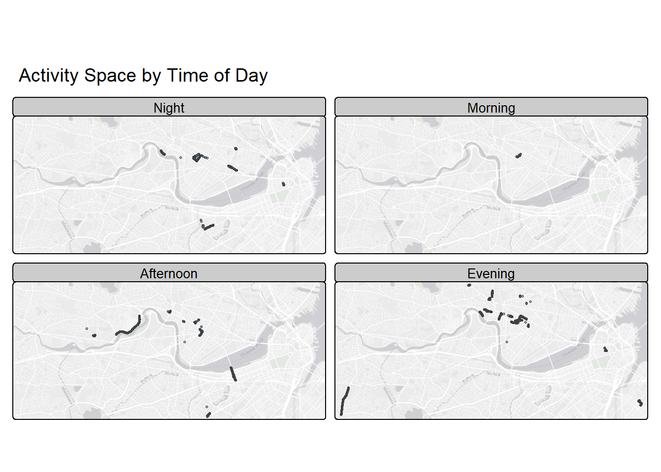

Interesting. I like the nightlife. I like to boogie.

🌿 Add Nature: Load up an NDVI Raster

Let’s make this a little richer by adding an environmental exposure that we could link to our data. Our old friend NDVI (Normalized Difference Vegetation Index) from Landsat (30m resolution) helps us understand greenness and vegetation density.

download.file("https://raw.githubusercontent.com/pjames-ucdavis/SPH215/refs/heads/main/NDVI_rast_boston.tif", destfile = "NDVI_rast_boston.tif", mode = "wb")
ndvi_raster <- rast("NDVI_rast_boston.tif")
ndvi_raster

## class       : SpatRaster 
## size        : 210, 583, 1  (nrow, ncol, nlyr)
## resolution  : 0.0002694946, 0.0002694946  (x, y)
## extent      : -71.19885, -71.04174, 42.33032, 42.38692  (xmin, xmax, ymin, ymax)
## coord. ref. : lon/lat WGS 84 (EPSG:4326) 
## source      : NDVI_rast_boston.tif 
## name        :  NDVI_mean 
## min value   : -0.1340106 
## max value   :  0.7256226

tm_shape(ndvi_raster) +
  tm_raster(col.scale = tm_scale_continuous(values = "brewer.yl_gn"),
            col.legend = tm_legend(title = "NDVI"))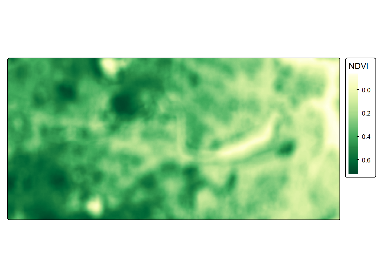

Looks quite green!

✨ Make It Beautiful with tmap

Time to show off with tmap, our old reliable thematic mapping package. We reproject the GPS points to match the raster and then we layer it all together.

tmap_mode("view")  # switch to interactive map mode

## ℹ tmap modes "plot" - "view"

# Reproject GPS CRS to match raster
gps_sf <- st_as_sf(gps_data, coords = c("longitude", "latitude"), crs = 4326)

# Transform our GPS CRS to match the raster!
gps_proj <- st_transform(gps_sf, crs = crs(ndvi_raster))


# Map it!
tm_shape(ndvi_raster) +
  tm_raster(col.scale = tm_scale_continuous(values = "brewer.yl_gn"),
            col_alpha = 0.55, 
            col.legend = tm_legend(title = "NDVI")) +
  tm_shape(gps_proj) +
  tm_symbols(
    fill = "blue", 
    size = 0.5, 
    col = NA,
    fill_alpha = 0.1
    ) +
  tm_title_out(title = "Where We've Been with a Little Green)")

## Registered S3 method overwritten by 'jsonify':
##   method     from    
##   print.json jsonlite

## Warning: tm_scale_intervals `label.style = "continuous"` implementation in view mode
## work in progress

Now we can visually inspect where I’ve been relative to greenness. This gives an idea of my actual exposure to greenness as I move through life. Slightly better than just residential address alone!

Extract NDVI values to GPS data

Finally, let’s extract NDVI values to GPS data to give us a quantitative estimate of where exactly we are exposed to greenspace. We will use the extract() function from the terra package to do this.

ndvi_values <- data.frame(gps_data,terra::extract(ndvi_raster, terra::vect(gps_proj)))
glimpse(ndvi_values)

## Rows: 21,264
## Columns: 18
## $ timestamp  <dbl> 1.61931e+12, 1.61931e+12, 1.61931e+12, 1.61931e+12, 1.61931…
## $ UTC.time   <dttm> 2021-04-25 00:15:10, 2021-04-25 00:16:58, 2021-04-25 00:16…
## $ latitude   <dbl> 42.37177, 42.37180, 42.37183, 42.37186, 42.37187, 42.37188,…
## $ longitude  <dbl> -71.08793, -71.08796, -71.08791, -71.08791, -71.08792, -71.…
## $ altitude   <dbl> 3.940258, 3.940258, 3.940258, 3.940258, 3.929049, 3.938418,…
## $ accuracy   <dbl> 65.00000, 1030.74153, 65.00000, 65.00000, 54.44491, 54.7162…
## $ time       <dttm> 2021-04-25 00:15:10, 2021-04-25 00:16:58, 2021-04-25 00:16…
## $ time_label <chr> "2021-04-25 00:15:10", "2021-04-25 00:16:58", "2021-04-25 0…
## $ lon2       <dbl> -71.08796, -71.08791, -71.08791, -71.08796, -71.08792, -71.…
## $ lat2       <dbl> 42.37180, 42.37183, 42.37186, 42.37183, 42.37188, 42.37188,…
## $ t2         <dttm> 2021-04-25 00:16:58, 2021-04-25 00:16:59, 2021-04-25 00:17…
## $ dt_s       <dbl> 108, 1, 1, 6, 1, 1, 1, 1, 1, 1, 1, 1, 1, 1, 1, 1, 1, 1, 1, …
## $ step_m     <dbl> 3.730937e+00, 5.242994e+00, 3.571994e+00, 5.394825e+00, 8.0…
## $ speed_mps  <dbl> 3.454572e-02, 5.242994e+00, 3.571994e+00, 8.991376e-01, 8.0…
## $ hour       <int> 0, 0, 0, 0, 0, 0, 0, 0, 0, 0, 0, 0, 0, 0, 0, 0, 0, 0, 0, 0,…
## $ tod        <fct> Night, Night, Night, Night, Night, Night, Night, Night, Nig…
## $ ID         <dbl> 1, 2, 3, 4, 5, 6, 7, 8, 9, 10, 11, 12, 13, 14, 15, 16, 17, …
## $ NDVI_mean  <dbl> 0.2657485, 0.2657485, 0.2624005, 0.2624005, 0.2624005, 0.26…

Look at the data

OK, and now we can take a glimpse at the data. This is one participant’s (me) minute-to-minute exposure to greenspace as they move throughout their lives. This is the full distribution of a personal exposure to NDVI for five days! If we had, for instance, physical activity data, we could see if momentary exposure to greenspace is associated with higher physical activity.

summary(ndvi_values$NDVI_mean)

##    Min. 1st Qu.  Median    Mean 3rd Qu.    Max. 
## 0.08799 0.33104 0.33498 0.33002 0.33498 0.64671

hist(
  ndvi_values$NDVI_mean,
  main = "Distribution of NDVI Exposure",
  xlab = "NDVI"
)

Exposure over time

Next, let’s take a look at how my exposure varies from minute to minute over the course of a few days. We can do that by simply plotting time and our GPS-based NDVI measure!

plot(
  ndvi_values$time,
  ndvi_values$NDVI_mean,
  type = "l",
  xlab = "Time",
  ylab = "NDVI",
  main = "Momentary Greenness Exposure"
)

Kinda like an EKG of greenness! Interesting!

🎉 You Did It!

You loaded real-world GPS data, estimated movement speed from raw GPS data, mapped it, extracted data from a vegetation raster, made it interactive, and created estimates of personal exposure. You now have the tools to link where people go to what they are exposed to. Pretty cool.

Over this quarter, we’ve taken our GIS data from the macro to the micro-scale. We’ve covered so much in so little time! You’ve learned a TON of R. It has been a mapping whirlwind, and I’m so proud of all of you!